From chemical kinetics to the Kimura Equation
There are many amazing beautiful papers that never catch on. I always felt John Tukey's 1950's papers on k-statistics 1 and 2 are somewhat underappreciated works of a creative genius. Tukey is, according to Wikipedia, "best known for the development of the fast Fourier Transform (FFT) algorithm and box plot".
(Ok, not to be rude, but does one really need to "develop" the box plot? It's... just a rectangle with sticks coming out of it.)
IMO, not exactly on the same level as the FFT (or k-statistics for that matter)
Counterwise, Daniel Gillespie's 1977 paper is one of those blockbusters that deserves the hype: clear, deep, and useful. It recaps his 1976 paper and shows a concrete example of what we now know as simply "the Gillespie algorithm" the simplest, most useful algorithm in the theory of stochastic processes. It's not really Gillespie's: just like the FFT (which we find in Gauss's unpublished work, 100 years before the first computer) isn't really Tukey's. Such a beautiful and useful algorithm can't be invented, only (re)discovered.
When I learn a topic, I try to find a satisfactory way to build it up analytically. That means choosing some starting point and then a series of tricks to get me to the most important equations. The 1977 paper is a good starting point: Gillespie has a clear description of the differential equations and combinatorics of stochastic processes. Although don't take his chemistry too seriously. Real chemistry is much more complicated.
The path I wish to take in this blog post is the path I've found to build up the Wright Equation. My goal is still to take us to population initialization for simulation purposes, but steps 3 and 4 still remain. We just get to the Kimura equation.
- Chemical reactions -> diffusion equation
- Balanced moran process -> Kimura equation
- Biallelic system -> Wright equilibrium
- Gibbs sampler -> Population initialization
Combinatorics of chemical reactions
Very generally we can describe a chemical reaction $i$ via it's stoichiometric coefficients
$$ \begin{equation} \sum_a {π^i_a} ·a \overset{λ_i}{\longrightarrow} \sum_b {ρ^i_b}·b \end{equation} $$
in a system with constant pressure and temperature, and flexible, impermeable walls. The system has $n_a$ well mixed particles of each type $a$.
This base rate is defined for each particular set of particles $π^i_a$, of each type $a$. Since we can choose any $π^i_a$ of the $n_a$ particles to take part, the total number of choices we can make to run a reaction is given by
$$ \begin{equation} h_i(\boldsymbol{n}) = \prod_a {n_a \choose{π_a^i} } \end{equation} $$
The symmetry factors of $\frac{1}{π_a!}$ in the binomial coefficients are important for keeping track of whether reactants are distinguishable. Important in the sense that you get the wrong answer if they are not there. I learned this the hard way: I once wrote down a chemical reaction system supposed to simulate clonal competition: in such cases there was a second-order reaction for self-competition:
$$ a + a \rightarrow a $$ and I missed this factor of 2 from the denominator of ${n_a \choose 2}$. This lead to some weird behavior and screwed up my carrying capacity. I had accidentally made self-competition twice as strong as non-self competition.
Why did that factor of 2 matter? We can imagine particles as swirling around a container with volume $V$. There is a particular tiny characteristic volume $v$ at which particles will be close enough to interact. If each of the $π_a^i$ are inside of that volume a reaction will take place at some rate $λ_v$.

reaction volumes are imaginary dotted lines in our container that sometimes contain enough particles to start a chemical reaction
The probability of that happening at any given moment is binomially distributed $$ \begin{aligned} p(π_a · a \in v) &= \prod_a {n_a \choose{π_a} } \left(\frac{v}{V}\right)^{π_a^i}\left(1-\frac{v}{V}\right)^{n_a-π_a^i} \\ &\approx \prod_a {n_a \choose{π_a} } \left(\frac{v}{V}\right)^{π_a^i}e^{-\frac{n_a v}{V}} \end{aligned} $$ Now consider self and non-self competition, they have the same same $v$, but their functional dependence is different: $$ \begin{aligned} p(a + a \in v) &= {n_a \choose{2} } \left(\frac{v}{V}\right)^{2}e^{-\frac{n_a v}{V}} & \text{self}\nonumber \\ p(a + b \in v) &= {n_a \choose{1} } {n_b \choose{1} } \left(\frac{v}{V}\right)^{2}e^{-\frac{(n_a +n_b) v}{V} } & \text{nonself}\nonumber \end{aligned} $$ You can convince yourself that, in the ideal gas limit, $\frac{(n_b+ n_a) v}{V}$ is (very) small. Thus, to first order, your dependence on reaction inputs $n_a$ is entirely in ${n_a \choose{π_a} }$. You can bundle everything else with your definition of the base reaction rate $λ_i$, but you have to keep track of ${n_a \choose{π_a} }$
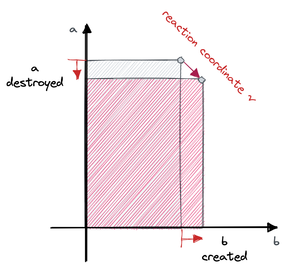
The total rate (the inverse-average-time to the next reaction) is then given by the product of the reaction multiplicity and the reaction rate. $$ a_i(\boldsymbol{n}) = λ_i h_i(\boldsymbol n) $$ What happens to the system state when a reaction goes? Each species $a$ changes number $n_a \rightarrow n_a + ρ_a - π_a$. We can think of $ρ^i_a - π^i_a = ν_a^i$ as being the $a$th component of the reaction coordinate vector $\boldsymbol ν$ so that $\boldsymbol n \rightarrow \boldsymbol n + \boldsymbol ν^i$.
This leads to the master equation, $$ \dot p(\boldsymbol n) = \sum_i a_i(\boldsymbol n - \boldsymbol ν^i)p(\boldsymbol n - \boldsymbol ν^i) - a_i(\boldsymbol n )p(\boldsymbol n) $$ representing the probability flux in (from $\boldsymbol n - \boldsymbol ν^i$), and out of the state defined by $\boldsymbol n$, summed over all reactions $i$
Now comes an elegant trick: to move to the continuum and get the diffusion equation: rewrite the shift operator as an exponential: $$ f(\boldsymbol n - \boldsymbol ν) = e^{- \boldsymbol ν · \boldsymbol ∂}f(\boldsymbol n) $$ The master equation then has the form $$ \begin{aligned} \dot p(\boldsymbol n) &= \sum_i \, ( e^{- \boldsymbol ν^i · \boldsymbol ∂}-1) a_i(\boldsymbol n )p(\boldsymbol n) \\ &\approx \sum_i \, - \boldsymbol ∂ · \boldsymbol ν^i ( a_i(\boldsymbol n )p(\boldsymbol n) )+\frac{1}{2} ( \boldsymbol ∂ ·\boldsymbol ν^i )^2 \left( a_i(\boldsymbol n )p(\boldsymbol n) \right) \end{aligned}$$ This is the diffusion equation representing the chemical reaction system composed of each reaction $i$. Following the notation in Risken, we identify two tensors, $D^{(1)}$ and $D^{(2)}$ for each reaction, $i$, the contribution to the drift and diffusion. $$ \begin{aligned} \dot{p}(\boldsymbol{n}) &= \sum_i \, - \boldsymbol ∂ · D^{(1)}_i p(\boldsymbol{n}) + \boldsymbol{∂}^2 · D^{(2)}_i p(\boldsymbol{n}) \end{aligned} $$
Balanced Moran process and Kimura Equation
Let's actually apply this equation to get the Fokker Planck equation for the balanced Moran process. I find the balanced Moran process generates lovely symmetrical and anti-symmetrical terms.
Let $e_a$ be the unit vector for the type $a$. A selection event in which $a \rightarrow b$ the balanced Moran process can be described by $$ \begin{aligned} a + b \overset{λ_{ab}}{\longrightarrow} a + a \\ a + b \overset{λ_{ba}}{\longrightarrow} b + b \end{aligned} $$ where we choose our rates in such a way as to make everything work out. $$ λ_{ab} = \frac{λ+f_a - f_b}{2N} \quad λ_{ba} = \frac{λ+f_b - f_a}{2N} $$ We have the condition which makes sampling fast that all pairs have the same total rate $$ λ_{ab} + λ_{ba} = \frac{λ}{N} \quad \forall a,b $$ Note that there are ${N \choose 2}$ pairs, so the total time until the next reaction is $\frac{N-1}{2λ}$. Every $\frac{N}{2λ}$ we draw two particles. The minus one comes because we ignore them if they are the same, otherwise we apply the selection operator. See the other blog post for details.
The reaction coordinates are given by $$ \boldsymbol ν^{ab} = \hat{e}_a - \hat{e}_b \quad \boldsymbol ν^{ba} = -\hat{e}_a + \hat{e}_b $$ while the total reaction wait time is $$ a_{ab}(\boldsymbol n) = λ_{ab} n_a n_b \quad a_{ba}(\boldsymbol n) = λ_{ba} n_a n_b $$
First we construct the contribution to the selection part of the drift tensor $D^{(1)}_s$ for each pair $a,b$. $$ \begin{aligned} D^{(1)}_{s_{ab}} (\boldsymbol n) &=\frac{1}{2}(\hat{e}_a - \hat{e}_b) (a_{ab}(\boldsymbol n) - a_{ba}(\boldsymbol n))\\ &= (\hat{e}_a - \hat{e}_b) (f_{a} - f_{b}) \frac{n_a n_b}{2N}\\ % &= \hat{e}_a n_a \frac{f_{a} n_b - n_b f_{b}}{N} + \hat{e}_b n_b \frac{ n_a f_{b} - n_a f_{a}}{N} \\ % D^{(1)}_s (\bm n) &= \sum_{(a,b)} D^{(1)}_{s(a,b)} (\boldsymbol n) \\ % &= \sum_{a} \hat{e}_a n_a (f_{a} - \overline f)\\ \end{aligned} $$
Now to get the diffusion equation, we again look at the forward and backward contribution to the diffusion equation from selection between each pair $(a,b)$, and you see the rates drop out $$ \begin{aligned} D^{(2)}_{s_{ab}} (\boldsymbol n) &=\frac{1}{4} (\hat{e}_a - \hat{e}_b) (\hat{e}_a - \hat{e}_b) (a_{ab}(\boldsymbol n) + a_{ba}(\boldsymbol n)) \\ &= (\hat{e}_a \hat{e}_a + \hat{e}_b\hat{e}_b - \hat{e}_a\hat{e}_b- \hat{e}_b\hat{e}_a ) n_a n_b \frac{ λ}{4N} \end{aligned} $$
Mutations
Now we look at the mutation operation $$ a \overset{μ_{ab}}{\longrightarrow} b \\ $$ Again the reaction coordinates are given by $$ \boldsymbol ν^{μ_{ab}} = \hat{e}_b - \hat{e}_a $$ This is a first order reaction (depends on only one input) and the total reaction rate is linear in particle number, $$ a_{μ_{ab}}(\boldsymbol n) = μ_{ab} n_a $$ We get our total drift tensor: $$ D_{μ_{ab}}^{(1)}(\boldsymbol n) = μ_{ab} n_a (\hat e_b - \hat e_a) \\ D^{(1)} =\sum_{ab} D_{μ_{ab}}^{(1)} + D_{s_{ab}}^{(1)} $$ The mutations don't happen fast enough to contribute much to the noise, so the diffusion tensor is just from the selection events $D^{(2)} = D_s^{(2)}$.
Coordinate transformation to frequency space
As promised, we now take the leap so that $x_a = \frac{n_a}{N}$. We then just use the coordinate transformation equation at the end of chapter 4 of Risken. Eq. 4.131 and 4.132: $$ \begin{align} D^{(1')}(\boldsymbol x) &= \sum_{a} \hat{e}_a \left( \frac{∂ x_a }{∂t} + \frac{∂ x_a }{∂ \boldsymbol n}·D^{(1)}_a + \frac{∂^2 x_a }{∂ \boldsymbol n ∂ \boldsymbol n} · D^{(2)} \right) \\ D^{(2')}(\boldsymbol x) &= \sum_{ab} \hat{e}_a \hat{e}_b \left( \frac{∂ x_a}{∂ \boldsymbol n}· D^{(2)}· \frac{∂ x_b }{∂ \boldsymbol n} \right) \end{align} $$ Since our coordinate transformation is linear we don't have to worry about the anomolous drift part, the $n_a$'s become $x_a$'s, painlessly $$ \begin{align} D^{(1')}(\boldsymbol x) &= (\hat{e}_a - \hat{e}_b) \left( (f_{a} - f_{b}) \frac{x_a x_b}{2} + μ_{ab} x_a \right) \\ D^{(2')}(\boldsymbol x) &= (\hat{e}_a \hat{e}_a + \hat{e}_b\hat{e}_b - \hat{e}_a\hat{e}_b- \hat{e}_b\hat{e}_a ) x_a x_b \frac{ λ}{4N} \end{align} $$ We did alright! Here's the full equation with the labels $a$ and $b$ interchanged to allow us to collect terms. $$ \begin{align} \dot p(\boldsymbol x) = \sum_{ab} \begin{cases} (∂_a x_a x_b - ∂_b x_a x_b) \frac{f_{a} - f_{b}}{2} p(\boldsymbol x)& \text{selection} \\ + μ_{ab} (∂_a x_a - x_a ∂_b)p(\boldsymbol x)& \text{mutation} \\ + \frac{ λ}{2N} (∂_a^2 x_a x_b - ∂_a ∂_b x_a x_b ) p(\boldsymbol x) & \text{drift} \end{cases} \end{align} $$ Where derivatives are here with respect to our new coordinates, the frequencies $x_a = n_a/N$, i.e. $∂_a = ∂/∂x_a$. It's tradition to use temporal units $2N_e$ where $N_e = N/λ$, with unitless terms $θ =2N_e μ$, and $σ = 2 N_e f$ $$ \begin{align} \dot p(\boldsymbol x) = \sum_{ab} \begin{cases} (∂_a x_a x_b - ∂_b x_a x_b) \frac{σ_{a} - σ_{b}}{2} p(\boldsymbol x) \\ + θ_{ab} (∂_a x_a - ∂_bx_a )p(\boldsymbol x) \\ + (∂_a^2 x_a x_b - ∂_a ∂_b x_a x_b ) p(\boldsymbol x) \end{cases} \end{align} $$ I like this form of the Kimura equation better than the one you see in textbooks. There's no if $a = b$, if $a\neq b$, like you see even in this nice paper, it's just a straight double sum over all pairs of genotypes. The lovely antisymmetry assures that the diffusion is confined to the simplex $\sum_a x_a = 1$. In accordance with that antisymmetry, the diagonal terms vanish. This beauty was inherited from the balanced Moran process I discuss here .
Evolution is an elegant process: a simple premise with literally endless implications. Its comforting to know that the fundamental diffusion equations of evolution can be cast in a form that carries at a hint of that elegance.
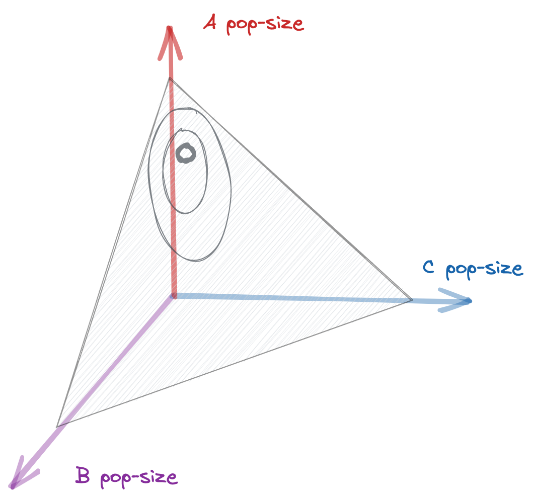
The Kimura equation defines a diffusion confined to the simplex over all population types