I'm going to walk through the code I use to implement the balanced Moran process in Julia. I thought I could just post the population dynamics part of this code, but the dynamics doesn't make much sense unless you know what everything is. So this ended up becoming an involved post about defining nice types in Julia for constructing and analyzing population simulations.

Look at the ffpopsim source code here. This is great code by great scientists, but the file haploid_high_d.h is a cool 1000 lines of well-commented but hard to read C++. Then it all gets stitched together with an enormous amount of Python. With Julia, I had some new ideas about the algorithm described below and rewrote it, from scratch in a single day. That's not because I'm a good programmer. This is the two language problem being solved.

So this post is as much about Julia code as about population simulation. I was motivated by Tim Holy's description of how Colors.jl can manipulate images at speed and in native Julia. Each pixel is a custom RGB type composed of three numbers, e.g.

struct RGBpixel
    red::Int8
    green::Int8
    blue::Int8
end

Coming from MATLAB, where structs are sluggish, the idea of making a whole image out of structs seemed absolutely ludicrous. But Tim assures us that, in fact, this is about the fastest way to do things in Julia. The key is that this object has no abstract references: it's just bits.

julia> a = RGBpixel(1,2,3)
RGBpixel(1, 2, 3)

julia> isbits(a)
true

This means that the compiler knows exactly how big a is. Thus, when you have an Array{RGBpixel}, the compiler allocates just enough memory for each little pixel. To the compiler it might as well be a vector of floats. Meaning: dense, strided and accessible as fast as your little processor can multiplex.

So this is our plan: make individuals be a type that has all the information we need, and make sure that this type satisfies isbits. Then our population is just a bunch of these dudes stored in a giant vector. In some ways it's a really dumb brute-force approach but it has a brutish elegance of its own and it's faster than you might think.

Code and descriptions

I hoped that you would be able to copy and paste all the code below in your Julia REPL to get your very own, very fast, endlessly flexible forward simulator. We're most of the way there, but the details of the initialization of the population and the mutational model must wait until another blog post because there's some interesting mathematics there that deserve some independent discussion.

Definition of the virus type

This is how I defined my individuals which I call Virus (thinking about HIV evolving within a patient)

struct Virus{G}
    genotype::G # heritable information
    parent_index::UInt # the parent birth index
    birth_index::UInt # birth ranking (virus ssn)
    birth_time::Float64 # when the virus was born
    death_time::Float64 # when it died
end

The birth and death times define the temporal extent of the virus's mortal coil (its worldline). The birth index is the virus's unique identifier and parent index is the identifier of the parent: what we need to reconstruct lineages--how it fits into the whole population tree.

I attach enough information to the virus to later be able to reconstruct everything. The entire population history. Overall this scheme sacrifices some speed for maximum flexibility in the analysis and model.

I'm agnostic about the type of the genotype-type G. G could be UInt8 for a tiny state space, or some long tuple or StaticArray of UInt64's for representing big genomes. As long as G is bits then Virus{G} will be bits to. If it is something more flexible, like an Array or BitVector, these have isbits == false and we will lose a lot of time, allocating and deallocating every event.

Constructing and changing viruses.

When a virus is born, you don't know the death_time yet. I set it to zero by default and use the SetField package to elegantly redefine a new version of the virus when it dies or gives birth to a copy of itself at a later time--its copy will require a new birth_index but the same genotype and birth time, hence set_birth_index.

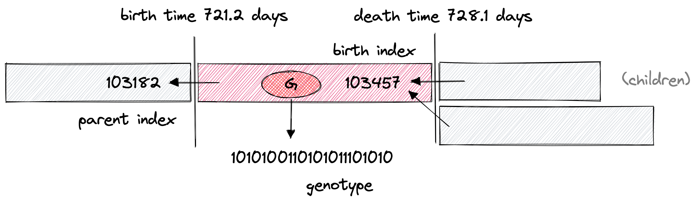
The components of a Julia type Virus{G}. — *How I visualize of the components of Virus{G}. The backward arrows indicate lineage relationships from the child to the parent. From these arrows, we can reconstruct the whole population tree.*

function Virus(genotype, parent_index, birth_index, birth_time;
    death_time = 0.0)
    # 0.0 is just a place holder until the virus dies
    Virus(genotype, parent_index, birth_index, birth_time, death_time)
end

using Setfield 
# helpful little package for copying a struct with one field changed.
function set_death(v::Virus, time)
    return @set v.death_time = time
end

function set_birth_index(v::Virus, birth_index)
    return @set v.birth_index = birth_index
end

You cant mutate immutable types, and you still can't:@set v.birth_index = birth_index is not mutation. Instead Setfield.jl destructs and restructs without you needing to worry about getting the constructor function signature right.

Definition of the population: living and the dead

The living and the dead depicted as volumes

A population is composed of two important vectors: the living vector is constant size, and the dead vector is of ever increasing size. As viruses die they get filed in the dead pile.

mutable struct Population{G}
    living::Vector{Virus{G}}
    dead::Vector{Virus{G}} # virus = pop.dead[birth_index] 
    next_birth::UInt # new viruses get a next birth as birth_index
    size::UInt # should stay length(individuals) == length(birth_time) etc
    time::Float64 # when the last event occured
end

I imagine the living and dead as two nested spheres. The dead is something like 120 gigapeople, the living 7 gigapeople. All of our ancestors falling in love, eating mammoths, discovering slood etc. The dead outnumber us and haunt us and deserve our respect. Ultimately, all human history will belong the the dead.

I look to pop.dead for the outcomes of the simulations: If I ask, "Was this or that phenotype at fixation at time $t$?" I just find all the viruses that were alive at $t$, and then check what their phenotype was.

Model parameters and fitness functions

We define a model by the potentially time-dependent bulk parameters, i.e.: fitness, mutation and drift. Drift is determined by $N_e$

struct DirichletModel{F}
    Ne::Float64
    incoming_rate::Vector{Float64} # incoming mutation rates
    fitness::F # f(g,t) fitness function of genotype and time
    nstates::UInt # number of states
    mutsample::Weights # amortized sampler
    total_rate::Vector{Float64}  # amortized sum
end

The fitness function is a mapping from genotype to fitness, and is one of the fields of our model struct.

Note how the fitness function type fitness::F is a free parameter F in the DirichletModel{F} type. This is because every function is it's own concrete type. With this pattern, there is no overhead to including the function as a struct field. I use this pattern often: build a closure and then include it inside a struct as a field, but there are other possible patterns to pass functions as parameters.

make the function a field in the struct with a unique free type parameter (as above).
make F a callable struct. This has the same behavior in that model.fitness(g,t) act's like a function, but you have finer control over what is saved. Less flexible but better guarantees e.g. to make sure that no global variables get captured.
make F a set of parameters for the fitness that then fitness(model, g, t) unpacks. This has the disadvantage that it creates an interface.

I will be looking at time-dependent fitness functions, and in general there is no finite set of parameters that will encode that feature, and this suggests the high flexibility of pattern (1).

In contrast, the mutation rates I'm interested in are usually constant. Therefore for the mutation process I went with (3) an interface. Mutational parameters are encoded in incoming_rate and total_rate, later unpacked by the interface functions mutation_wait and mutation_flip which generates the mutation Markov chain. In the end, you need to implement the following functions on the genotypes to make a new mutational model type work

mutation_wait(genotype, model) # -> time to next mutation event
mutation_flip(old_genotype, model) # -> new genotype
# generates a vector of tuples for the virus history (t1,g1),(t2,g2)
generate_initial_population(model; pop_size = 1)
# generates an initial batch of genotypes from the equilibrium distribution to start the population out.

Jointly, mutation_wait and mutation_flip define the continuous time markov process for the mutations.

Interfaces are flexible, but they require really good documentation to use. You have to know exactly what kind of methods are needed: what they are named, and what they should do.

Initialization

We use the generate_initial_population method to generate the initial population from the equilibrium distribution.

function initial_population(individuals::Vector{G}, model; 
time = 0.0) where G
    living = Vector{Virus{G}}()
    dead = Vector{Virus{G}}()
    next_birth = one(UInt)
    size = zero(UInt)
    birth_perm = UInt[]
    for i in individuals
        v = Virus(i, zero(UInt), next_birth, time)
        push!(living, v)
        size += 1
        next_birth += 1
    end
    Population{G}(living, dead, next_birth, size, time, birth_perm)
end

function initial_population(model; time = 0.0, pop_size = 1.0, λ = pop_size/model.Ne) where G
    individuals = generate_initial_population(model; pop_size)
    return initial_population(individuals, model; time)
end

There will be more on the Gibbs sampling step in generate_initial_population in another blog post.

Dynamics

We mutate the viruses using mutation_wait and mutation_flip. We then store the viruses in with the dead at the position birth_index and with the death time (see record death!).

function record_death!(pop, v0, t)
    if length(pop.dead) < v0.birth_index
        resize!(pop.dead, v0.birth_index)
        # make sure we are never out of bounds
    end
    pop.dead[v0.birth_index] = set_death(v0, t)
end

function step_mutation(v0::Virus{G}, pop, model) where G
    g::G = v0.genotype
    t = v0.birth_time + mutation_wait(g,model) 
    if t < pop.time
        g = mutation_flip(g,model) 
        # generate a new genotype
        # use the mutation time
    else
        t = pop.time 
        # use end time 
        # use old type genotype
    end
    record_death!(pop, v0, t)
    v0 = Virus(g, v0.birth_index, pop.next_birth, t) # create a daughter cell with the new features
    pop.next_birth += 1
    return v0
end

function update_mutations!(pop::Population, index, model)
    v0 = pop.living[index] # get the mutating virus
    while true
        v0 = step_mutation(v0, pop, model)
        if v0.birth_time == pop.time 
        # if the virus is up-to-date
            return v0
        end
    end
end

We want it so that both viruses in the balanced-Moran process have experienced the full cumulative effect of mutations when they come into battle. We're making no assumptions about a separation of time scales, e.g. mutations being slow and fitnesses being fast.

We also want them to be born at the same time so that they are exchangeable on the family tree.

update_mutations! accomplishes both, bringing the virus worldlines into synch. This means, that either can be the parent of the other. This is depicted graphically in second step of the figure below.

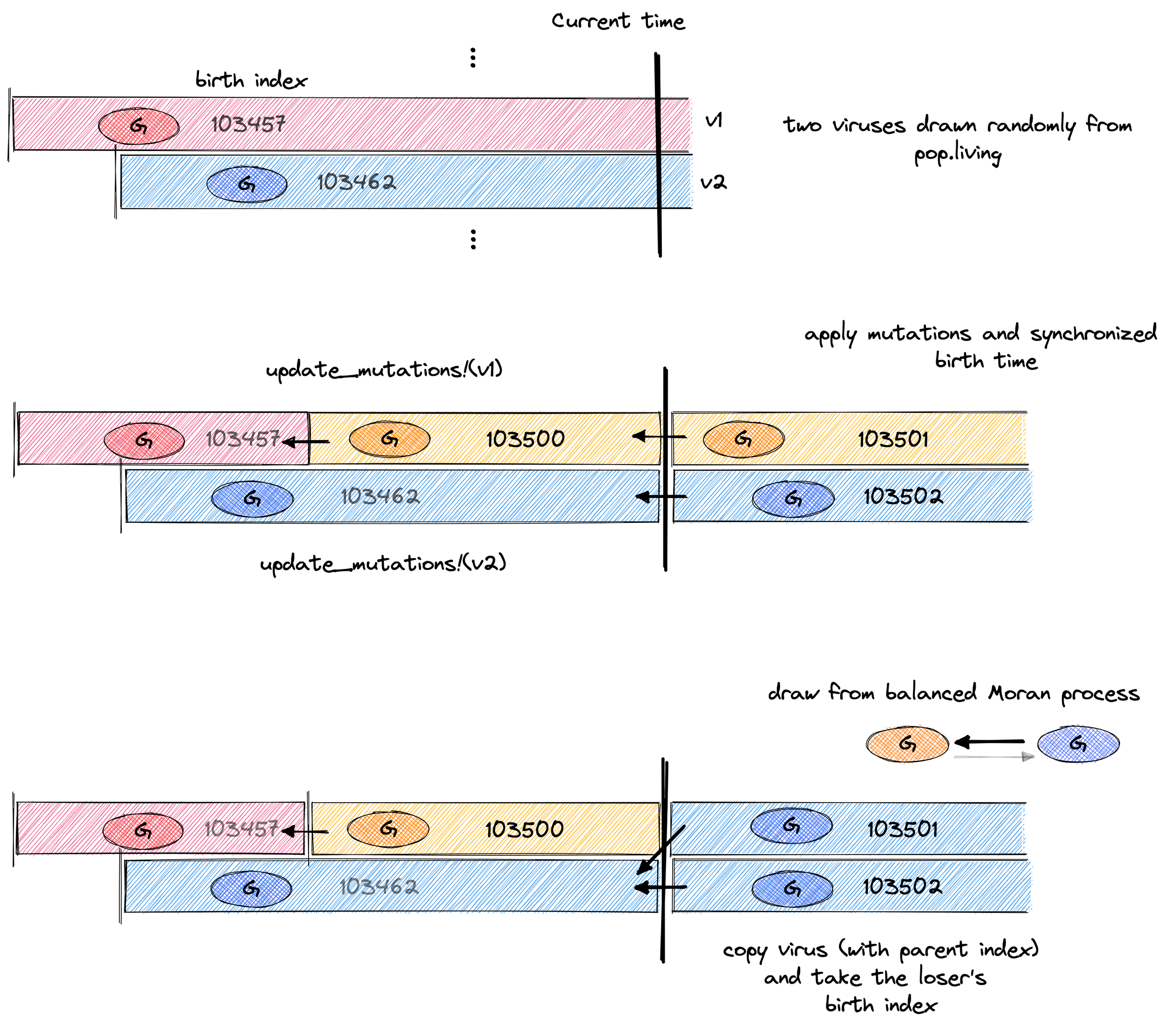
*A visual description of what’s happening in the code below. Virus* `103462` *with the blue phenotype wins the above battle and becomes the proud parent of* `103501` *and* `103502`!

Now we come to the core dynamics of a single selection event. Here, things are extremely straightforward: draw two viruses, calculate their fitness, chose one to live, one to die and set_birth_index accordingly.

function sample_bernoulli_fitness(f1,f2,λ) 
    # we includ
    if abs(f1 - f2) > λ 
        error("fitness out of bounds:\n f=$f , φ=$φ, λ= $λ ")
    end
    p = (1 + (f1 - f2)/λ)/2
    return rand(Bernoulli(p))
end


function selection_event!(pop::Population, model; λ = pop.size/model.Ne)
    i1 = rand(1:pop.size)
    i2 = rand(1:pop.size)
    if i1 != i2
        v1 = update_mutations!(pop, i1, model) 
        v2 = update_mutations!(pop, i2, model)
        f1 = model.fitness(v1.genotype, pop.time)
        f2 = model.fitness(v2.genotype, pop.time)
        t12 = sample_bernoulli_fitness(f1,f2,λ)
        if t12 # if i1 lives and and i2 dies
            pop.living[i1] = v1
            pop.living[i2] = set_birth_index(v1, v2.birth_index) # make a sibling with the same properties but a new index
        else # if i1 dies and and i2 lives
            pop.living[i1] = set_birth_index(v2, v1.birth_index)
            pop.living[i2] = v2
        end
    end
end

function pop_step!(pop::Population, model; λ = pop.size/model.Ne)
    pop.time += 2 * randexp() / (λ * pop.size)
    selection_event!(pop, model; λ)
end

function time_evolve!(pop::Population, model; λ = pop.size/model.Ne, final_time = 1.0)
    while pop.time < final_time
        pop_step!(pop, model; λ)
    end
end

function kill_population!(pop::Population{G}) where G
    for v in pop.living
        record_death!(pop, v, pop.time)
    end
    pop.living = Virus{G}[]
end

Conclusions

This is not the absolute fastest algorithm for any situation. For instance, a common alterntaive is to use clone counting instead of individual viruses. At low mutation rates and small genotypes, there is a lot of degeneracy and we rarely need to do anything but increment or decrement the clone size parameter. We can leverage the indistinguishability of clones to more efficiently apply our mutation operator. But there are a couple of things to highlight about this algorithm and this implementation that I think are quite nice:

This code is completely exact in that the selection events and mutation events are drawn from a continuous-time markov model, exactly specified by the rate model. This means we can explore a wider parameter space with a warm fuzzy feeling of mathematical precision.
We have stored every detail in the population evolution, and this helps us study the complete dendrochronology of our population. For instance, if we wanted to simulate the effect of strong selection on the neutral diversity, like with Alison Feder's cool paper, we can get exact values of θ from the trees, without every needing to keep track of a single neutral site at the genotype level. We have the statistical precision offered by an infinite number of neutral sites.
Finally look at the profiling: we can see a surprising amount of fundamental operations. Indexing and allocating comes in at only around 30% the total time spent. For keeping full tree information, that is really good.

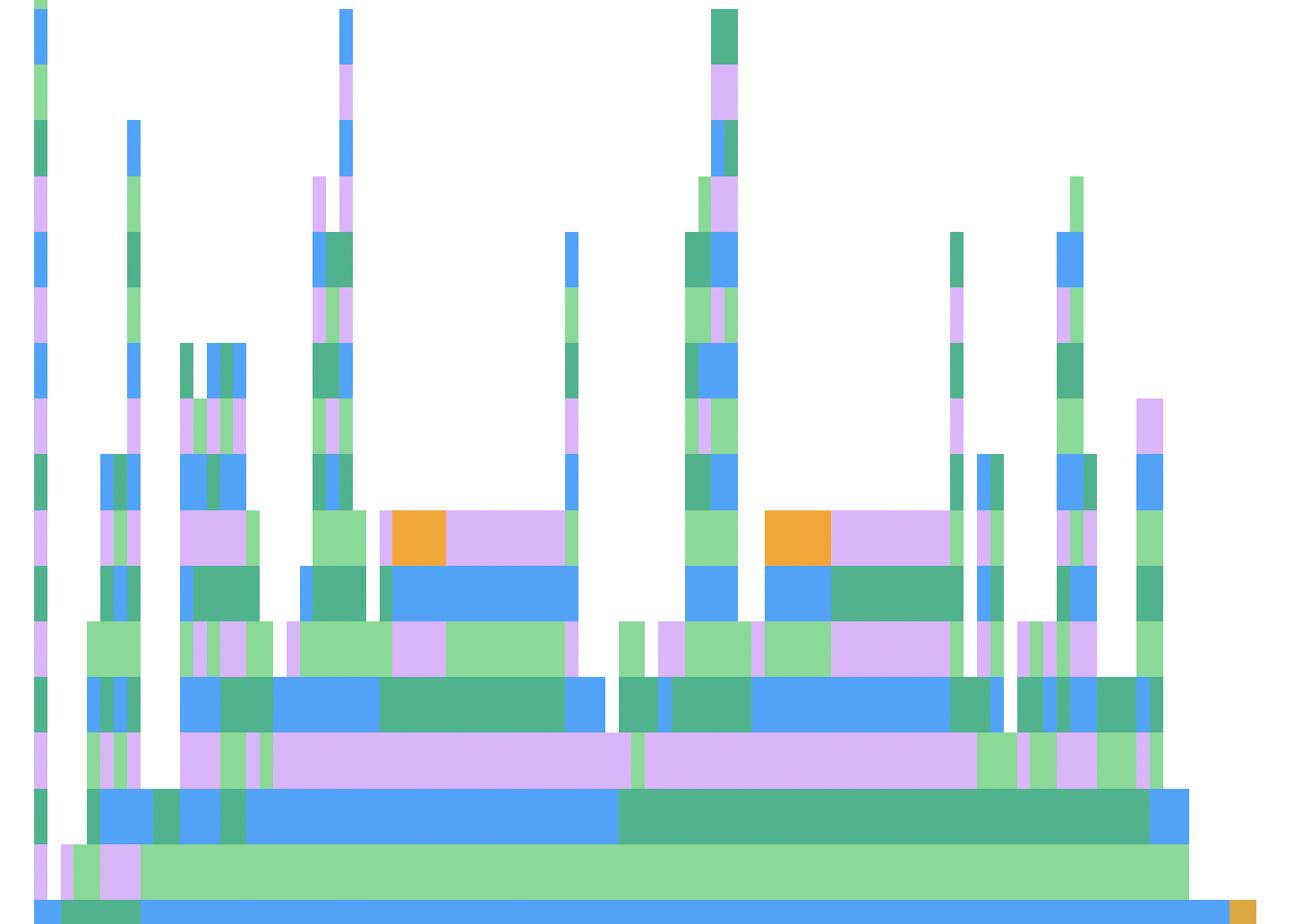
These candyland spires are a good sign that the code is tastes good to a CPU, although it doesn’t mean there isn’t a better algorithm that takse advantage of clone counting. This is generated by ProfileViews.jl

These kind of "candyland spires" profile views are a good sign that the code is near optimal for this particular algorithm. Those towers are the profiler hitting rands(). Red and orange plateaus are a sign that the code is stuck playing with types or memory instead of generating random numbers. We only have a little bit of orange from storing everything in pop.dead On a single thread of my 2017 i7 Macbook, I can generate and store $10^9$ UInt64 viruses in 60 seconds with time-varying fitness.

But the nicest thing is not having to decide on observables at runtime, but being able to read from the complete edition of the Book of Life. The combination of flexibility and speed of this approach is hard to beat.

Fast forward simulations of populations in Julia